RNN (Recurrent Neural Network)

RNN

python

Text generation with RNN

Author

ujjal

Published

June 27, 2023

RNN (Recurrent Neural Network)

A RNN is a type of artificial neural network which uses sequential data or time series data
A RNN is a several copy of same neural network that are aligned togther and each one passes its output to the next one
Each copy call timestep because it receives different input at different time step
RNN are call recurrent because they perform the same task for every element of a sequence.
RNN have a memory which capture information about what has been calculated so far #### Application
Rnn are used for time series analysis
when we need to make a predction based on previous data, not only current data

Problems of standard network:

Inputs, outputs can be different lengths in different examples.
Doesn’t share features learned across different positions of text.

Types of RNN:

one-to-one
one-to-many
many-to-one
many-to-many

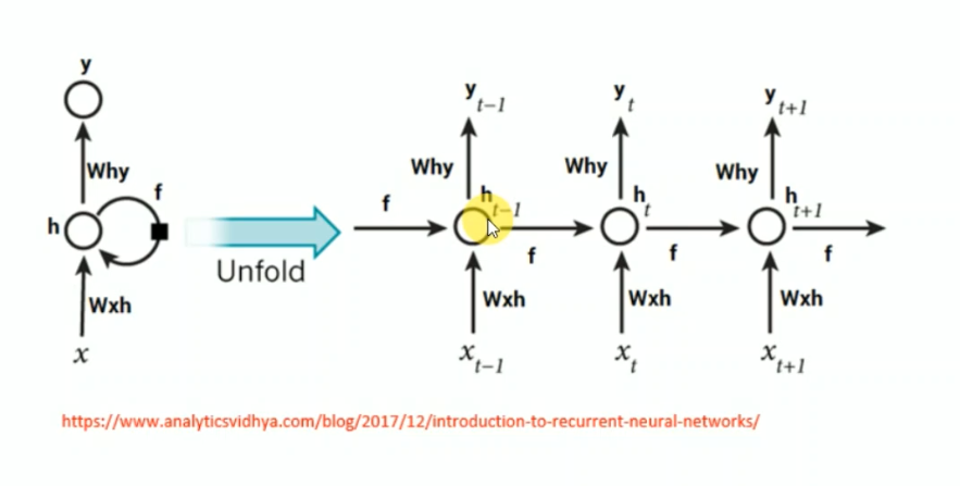
Unfolding RNN

RNN backpropagation through time

forward pass

Backword pass

The BPTT algorithm is used to calculate the gradients of the loss with respect to the parameters of the RNN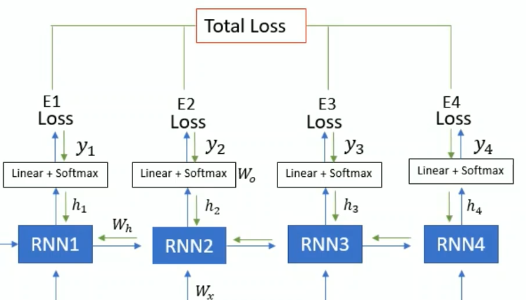

first calculate gradient with respect to (\(w_0\))
\[\frac{\mathrm{d}E_1}{\mathrm{d}W_0} = \frac{\mathrm{d}E_1}{\mathrm{d}y_1} \frac{\mathrm{d}y_1}{\mathrm{d}W_0}\] \[\frac{\mathrm{d}E_2}{\mathrm{d}W_0} = \frac{\mathrm{d}E_2}{\mathrm{d}y_2} \frac{\mathrm{d}y_2}{\mathrm{d}W_0}\] \[\frac{\mathrm{d}E_3}{\mathrm{d}W_0} = \frac{\mathrm{d}E_3}{\mathrm{d}y_3} \frac{\mathrm{d}y_3}{\mathrm{d}W_0}\] \[\frac{\mathrm{d}E_4}{\mathrm{d}W_0} = \frac{\mathrm{d}E_4}{\mathrm{d}y_4} \frac{\mathrm{d}y_4}{\mathrm{d}W_0}\]

All RNN unit have same weights

calculate gradient with respect to recurrent weights(\(w_h\))

\[\frac{\mathrm{d}E_1}{\mathrm{d}W_h} = \frac{\mathrm{d}E_1}{\mathrm{d}y_1} \frac{\mathrm{d}y_1}{\mathrm{d}h_1} \frac{\mathrm{d}h_1}{\mathrm{d}W_h}\] \[\frac{\mathrm{d}E_2}{\mathrm{d}W_h} = \frac{\mathrm{d}E_2}{\mathrm{d}y_2} \frac{\mathrm{d}y_2}{\mathrm{d}h_2} \frac{\mathrm{d}h_2}{\mathrm{d}W_h}\] we know in RNN current recurrent unit depedent on previous recurrent unit. so \(h_2\) depedent on \(h_1\). so the formula is- \[\frac{\mathrm{d}E_2}{\mathrm{d}W_h} = \frac{\mathrm{d}E_2}{\mathrm{d}y_2} \frac{\mathrm{d}y_2}{\mathrm{d}h_2} \frac{\mathrm{d}h_2}{\mathrm{d}h_1} \frac{\mathrm{d}h_1}{\mathrm{d}w_h} + \frac{\mathrm{d}E_2}{\mathrm{d}y_2} \frac{\mathrm{d}y_2}{\mathrm{d}h_2} \frac{\mathrm{d}h_2}{\mathrm{d}W_h}\] similar \[\frac{\mathrm{d}E_3}{\mathrm{d}W_h} = \frac{\mathrm{d}E_3}{\mathrm{d}y_3} \frac{\mathrm{d}y_3}{\mathrm{d}h_3} \frac{\mathrm{d}h_3}{\mathrm{d}w_h} + \frac{\mathrm{d}E_3}{\mathrm{d}y_3} \frac{\mathrm{d}y_3}{\mathrm{d}h_3} \frac{\mathrm{d}h_3}{\mathrm{d}h_2} \frac{\mathrm{d}h_2}{\mathrm{d}w_h} + \frac{\mathrm{d}E_3}{\mathrm{d}y_3} \frac{\mathrm{d}y_3}{\mathrm{d}h_3} \frac{\mathrm{d}h_3}{\mathrm{d}h_2} \frac{\mathrm{d}h_2}{\mathrm{d}h_1} \frac{\mathrm{d}h_1}{\mathrm{d}w_h}\]

Stacking RNN Layers

The output of the first RNN is passed to another RNN. Therefore the top-RNN receives the hidden state of the first RNN

Challenges in RNN

Vanising Gradient - gradient can be very low. It refers to the issue where the gradients calculated during backpropagation become extremely small as they are propagated backward through time, leading to very slow or ineffective learning.

The vanishing gradient problem can have several consequences:

Difficulty in Capturing Long-Term Dependencies: RNNs are designed to capture dependencies over long sequences. However, when the gradients vanish, the network struggles to propagate information over many time steps, limiting its ability to capture long-term dependencies
Slow Learning: With vanishing gradients, the network learns at a slow pace since the weight updates in the early layers are negligible \[\frac{\mathrm{d}E_3}{\mathrm{d}W_h} = \frac{\mathrm{d}E_3}{\mathrm{d}y_3} \frac{\mathrm{d}y_3}{\mathrm{d}h_3} \frac{\mathrm{d}h_3}{\mathrm{d}h_2} \frac{\mathrm{d}h_2}{\mathrm{d}h_1} \frac{\mathrm{d}h_1}{\mathrm{d}w_h} +....+\] lets \[\frac{\mathrm{d}E_3}{\mathrm{d}y_3} = 0.3 \frac{\mathrm{d}y_3}{\mathrm{d}h_3}=0.2 \frac{\mathrm{d}h_3}{\mathrm{d}h_2} = 0.5 \frac{\mathrm{d}h_2}{\mathrm{d}h_1} = 0.08 \frac{\mathrm{d}y_1}{\mathrm{d}w_h}=0.01\]

So \(\frac{\mathrm{d}E_3}{\mathrm{d}W_h} = 0.3*0.2*0.5*0.08*0.01 = 0.0002\) almost 0

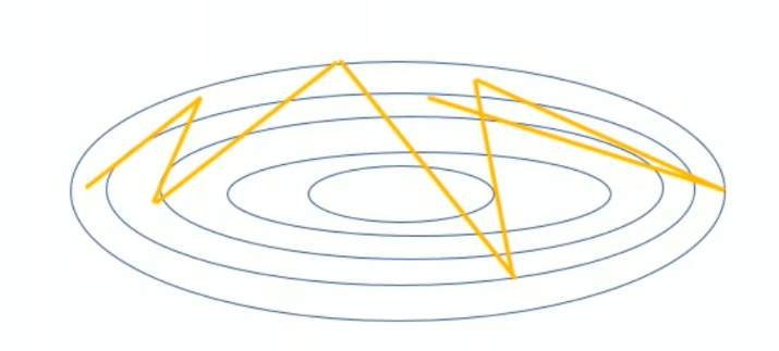
Exploding Gradient - Gradient can be very large , cause the loss and weiget update to heavily fluctuate

Solution for Exploding Gradient problem

Gradient Clipping: clip the Gradient to spacific value the exceed a spacific threshold if gradients exceed to 5, then clip to 0.2

import torch
import torch.nn as nn
import numpy as np

class DictnaryEmbd(object):
    def __init__(self):
        self.idx = 0
        self.idx2word = {}
        self.word2idx = {}
    def addword(self,word):
        if word not in self.word2idx:
            self.idx2word[self.idx] = word
            self.word2idx[word] = self.idx
            self.idx += 1
    def __len__(self):
        return len(self.word2idx)

class Textpreprocess(object):
    def __init__(self):
        self.dict_embd = DictnaryEmbd()
    def get_data(self,file_path,batch_size):
        len_word = 0
        with open(file_path,'r') as f:
            for line in f:
                words = line.split() + ['<eos>']
                for w in words:
                    self.dict_embd.addword(w)
                    len_word += 1
        tensor = torch.LongTensor(len_word)
        with open(file_path,'r') as f:
            ind = 0
            for line in f:
                words = line.split() + ['<eos>']
                for w in words:
                    tensor[ind] = self.dict_embd.word2idx[w]
#         print(tensor.shape)
        num_batches = tensor.shape[0]//batch_size
        tensor = tensor[:batch_size*num_batches]
        tensor= tensor.view(batch_size,-1)
        return tensor

corpus = Textpreprocess()
tensor = corpus.get_data('alice.txt',20)
tensor.shape

torch.Size([20, 1484])

embed_size = 128   
hidden_size = 1024 
num_layers = 1
num_epochs = 20
batch_size = 20
timesteps = 30
learning_rate = 0.002